
Handling Imbalanced Datasets in Python: SMOTE, Class Weights, and Math Explained
Handling imbalanced datasets requires overcoming the accuracy paradox by either penalizing minority misclassifications more heavily (class weighting via cost-sensitive loss), synthetically expanding the minority feature space (SMOTE via k-nearest neighbor linear interpolation), or adjusting the classification boundary (threshold moving). Model performance must be evaluated using Precision-Recall curves and F1-scores rather than raw accuracy or ROC-AUC.
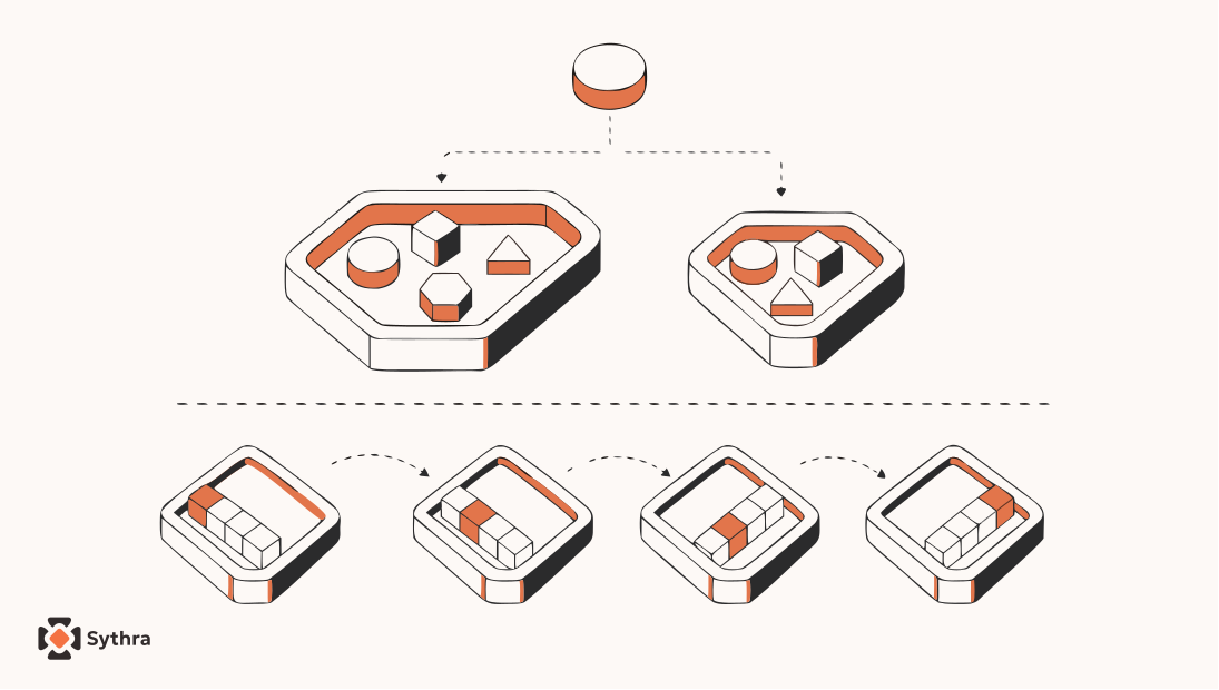
In machine learning classification, an imbalanced dataset occurs when the distribution of target classes is severely skewed — where a majority class represents the overwhelming bulk of the data (e.g., 99% legitimate transactions, 99.5% healthy patients), while the class of genuine interest (fraud, rare disease, equipment failure) constitutes a tiny fraction. When trained on skewed data, standard algorithms fall victim to the Accuracy Paradox: they maximize overall mathematical accuracy by simply predicting the majority class for every sample, quietly rendering the model useless for the exact task it was built to solve.
1. Key Concepts & Definitions
Handling class imbalance requires attacking the problem from one of three distinct architectural angles: altering the loss penalty (Class Weighting), generating synthetic data points (SMOTE), or altering the post-training decision cutoff (Threshold Moving). Before examining the mathematics, let us define the core terminology in plain English:
| Term / Parameter | Mathematical Role | Plain-English Intuition | Impact on Model Behavior |
|---|---|---|---|
| Imbalance Ratio (IR) | The ratio of majority examples to minority examples. | indicates moderate imbalance; requires dedicated cost-sensitive or resampling remediation. | |
| Class Weight () | Multiplier applied to sample loss: | A punitive fine scale: mistakes on rare classes cost significantly more. | Forces gradient descent updates to pivot toward correctly separating rare minority instances. |
| SMOTE | Linear interpolation: | Creates synthetic 'clones with variation' between real minority neighbors. | Expands the physical volume and density of the minority decision region in feature space. |
| Interpolation Dial () | Random scalar drawn uniformly from | A percentage slider along the straight line between two neighbors. | places a synthetic point exactly midway between two real observations. |
| PR-AUC (Average Precision) | Area under the Precision-Recall curve | Measures precision across all recall levels without being diluted by True Negatives. | The gold-standard evaluation metric for imbalanced data (unlike ROC-AUC, which masks false alarms). |
| Threshold Moving () | Classify positive if (default ) | Lowering the bar of suspicion to catch more rare cases. | Increases recall at the cost of precision without needing retraining or dataset alteration. |
2. Method 1: Class Weighting & Cost-Sensitive Loss
Standard machine learning models treat every training observation identically. In standard Binary Cross-Entropy (Log Loss) for logistic regression, the cost function over training examples is:
When 99% of samples belong to class 0 (), the right-hand term completely dominates the loss summation. The optimizer can slash total cost almost to zero by simply shifting the bias strongly negative so that everywhere, completely ignoring the 1% of minority points.
The Weighted Cost Function
Class weighting introduces a per-class loss multiplier , scaling the penalty based on the ground-truth label of sample :
The standard, principled approach adopted by Scikit-Learn (via class_weight='balanced') sets these weights inversely proportional to class frequencies:
Where is the total dataset size, is the number of classes ( for binary classification), and is the number of samples in class .
When computing gradient updates during gradient descent, this scalar weight flows directly into the parameter gradient:
If class 1 is 9 times rarer than class 0 (e.g., 90 healthy vs 10 sick): , while . A misclassification on a sick patient pulls the weights 9 times harder () than a mistake on a healthy patient, forcefully steering the decision boundary toward protecting the rare class.
3. Method 2: SMOTE Math & Geometry
Rather than modifying the loss function, SMOTE (Synthetic Minority Oversampling Technique) balances the dataset by generating synthetic minority examples directly within the feature space. Crucially, SMOTE does not create exact duplicates of existing points (which would cause severe overfitting to individual noise points). Instead, it draws synthetic samples along the line segments connecting existing minority points to their nearest minority neighbors.
The SMOTE Algorithm Step-by-Step
- Identify the Minority Set: Isolate all minority class observations .
- Find k-Nearest Neighbors: For each minority observation , compute the Euclidean distance to all other points in , and identify its nearest neighbors (typically ).
- Sample a Neighbor: Randomly select one neighbor from those nearest neighbors.
- Sample an Interpolation Dial: Draw a random scalar .
- Synthesize the New Observation: Create the synthetic point along the connecting vector:
Geometrically, is the directional vector extending from to . Multiplying this vector by scales it to an intermediate segment. Adding this back to produces an entirely new point that resides firmly within the plausible topological region of the minority class.
4. Method 3: Threshold Moving (The Zero-Cost Alternative)
Probabilistic binary classifiers (such as Logistic Regression, Random Forests, and Gradient Boosting) output a continuous predicted probability . By default, libraries apply a decision cutoff of :
The cutoff inherently assumes that a False Positive (false alarm) and a False Negative (missed case) carry identical costs. In imbalanced problems, this assumption is false. Missing a fraudulent transaction or a malignant tumor is orders of magnitude more expensive than flagging a legitimate user for verification.
Threshold Moving shifts to optimize a specific objective (such as maximizing the F1-score or minimizing asymmetric financial loss) without altering training data or model weights:
If missing a fraud incident costs while checking a false positive costs , the optimal decision threshold drops to . Lowering the threshold to forces the model to flag cases whenever there is even a 2% suspicion, dramatically boosting minority recall instantly.
5. Why ROC-AUC Fails (And Why PR-AUC Is Required)
A pervasive mistake in machine learning is evaluating imbalanced models using the standard Receiver Operating Characteristic (ROC-AUC) curve. ROC curves plot the True Positive Rate (Recall) against the False Positive Rate (FPR):
Examine the denominator of : it contains (True Negatives). In a dataset with 99,000 negatives and 1,000 positives, if the model generates 1,000 false alarms () while catching 800 positives ():
- The ROC curve looks outstanding, yielding an AUC of because the massive number of True Negatives dwarfs the False Positives.
- However, compute Precision: More than half of all alerts are false alarms!
PR-AUC (Precision-Recall Area Under Curve / Average Precision) does not include True Negatives in either axis. It focuses exclusively on the minority class performance, providing an honest, uninflated evaluation of model effectiveness under heavy skew.
6. From-Scratch Python Implementation (NumPy)
Let us implement both SMOTE's geometric interpolation algorithm and a Class-Weighted Logistic Regression training loop from scratch using pure NumPy.
import numpy as np

def smote_from_scratch(X_minority, n_samples_to_generate, k=5, random_state=42):
    """
    Generates synthetic samples by interpolating between minority seed points
    and their k-nearest neighbors in Euclidean feature space.
    """
    rng = np.random.default_rng(random_state)
    n_minority, n_features = X_minority.shape
    synthetic = np.empty((n_samples_to_generate, n_features))

    for i in range(n_samples_to_generate):
        # 1. Randomly choose a minority seed point
        seed_idx = rng.integers(0, n_minority)
        x_seed = X_minority[seed_idx]

        # 2. Find Euclidean distance to all other minority observations
        distances = np.linalg.norm(X_minority - x_seed, axis=1)
        distances[seed_idx] = np.inf  # Exclude self-distance

        # 3. Identify k nearest neighbors and pick one at random
        effective_k = min(k, n_minority - 1)
        k_nearest_indices = np.argpartition(distances, effective_k)[:effective_k]
        neighbor_idx = rng.choice(k_nearest_indices)
        x_neighbor = X_minority[neighbor_idx]

        # 4. Generate new point along connecting line segment
        lam = rng.uniform(0.0, 1.0)
        synthetic[i] = x_seed + lam * (x_neighbor - x_seed)

    return synthetic


def sigmoid(z):
    return 1.0 / (1.0 + np.exp(-np.clip(z, -250, 250)))


class WeightedLogisticRegressionScratch:
    """
    Cost-sensitive Logistic Regression with sample weights inversely proportional
    to class frequencies: omega_c = m / (K * m_c).
    """
    def __init__(self, lr=0.1, n_iters=1500):
        self.lr = lr
        self.n_iters = n_iters
        self.w = None
        self.b = 0.0

    def fit(self, X, y):
        m, n = X.shape
        self.w = np.zeros(n)
        self.b = 0.0

        # Compute balanced class weights
        classes, counts = np.unique(y, return_counts=True)
        K = len(classes)
        weight_map = {c: m / (K * count) for c, count in zip(classes, counts)}
        sample_weights = np.array([weight_map[label] for label in y])

        # Gradient descent optimization
        for _ in range(self.n_iters):
            z = X @ self.w + self.b
            y_pred = sigmoid(z)

            # Weighted gradient calculation
            error = (y_pred - y) * sample_weights
            dw = (1.0 / m) * (X.T @ error)
            db = (1.0 / m) * np.sum(error)

            self.w -= self.lr * dw
            self.b -= self.lr * db

        return self

    def predict_proba(self, X):
        return sigmoid(X @ self.w + self.b)

    def predict(self, X, threshold=0.5):
        return (self.predict_proba(X) >= threshold).astype(int)


# Verification test on synthetic imbalanced data (90:10 ratio)
if __name__ == "__main__":
    rng = np.random.default_rng(42)
    # Class 0: 90 majority points around (0, 0)
    X_0 = rng.normal(loc=0.0, scale=1.0, size=(90, 2))
    # Class 1: 10 minority points around (2.5, 2.5)
    X_1 = rng.normal(loc=2.5, scale=1.0, size=(10, 2))

    X = np.vstack([X_0, X_1])
    y = np.array([0] * 90 + [1] * 10)

    # Generate 80 synthetic minority observations to achieve a 1:1 balance
    X_synthetic = smote_from_scratch(X_1, n_samples_to_generate=80, k=4)
    print(f"Original shape: {X.shape}, Synthetic points created: {X_synthetic.shape}")

    # Fit weighted model
    model = WeightedLogisticRegressionScratch(lr=0.05, n_iters=2000)
    model.fit(X, y)
    preds = model.predict(X)
    print(f"Learned weights w: {np.round(model.w, 3)}, Bias b: {round(model.b, 3)}")
    print(f"Minority Recall on Training Set: {np.sum((preds == 1) & (y == 1)) / 10:.2f}")
7. Production Scikit-Learn & Imblearn Pipeline (Preventing Data Leakage)
When implementing SMOTE in real-world systems, the most widespread bug is data leakage during cross-validation. If you apply SMOTE to the whole dataset before splitting into folds, synthetic samples generated from test-fold points end up in the training fold. The model is evaluated on test instances that it effectively already memorized during synthesis, producing dishonestly optimistic performance metrics.
Here is the production-ready script benchmarking four approaches on an imbalanced dataset (95% majority, 5% minority):
import numpy as np
from sklearn.datasets import make_classification
from sklearn.model_selection import train_test_split
from sklearn.linear_model import LogisticRegression
from sklearn.metrics import classification_report, average_precision_score
from imblearn.over_sampling import SMOTE
from imblearn.pipeline import Pipeline as ImbPipeline

# 1. Synthesize an imbalanced dataset (95:5 ratio, 2,000 samples)
X, y = make_classification(
    n_samples=2000,
    n_features=10,
    n_informative=6,
    weights=[0.95, 0.05],
    flip_y=0.01,
    random_state=42
)

# Always stratify split so train and test preserve the 95:5 ratio
X_train, X_test, y_train, y_test = train_test_split(
    X, y, test_size=0.25, stratify=y, random_state=42
)

print(f"Train class distribution: {np.bincount(y_train)} (95% vs 5%)")
print(f"Test class distribution:  {np.bincount(y_test)}")

# --- Approach 1: Unweighted Baseline ---
model_baseline = LogisticRegression(random_state=42)
model_baseline.fit(X_train, y_train)
y_prob_baseline = model_baseline.predict_proba(X_test)[:, 1]
y_pred_baseline = model_baseline.predict(X_test)

# --- Approach 2: Cost-Sensitive Class Weighting ---
model_weighted = LogisticRegression(class_weight="balanced", random_state=42)
model_weighted.fit(X_train, y_train)
y_prob_weighted = model_weighted.predict_proba(X_test)[:, 1]
y_pred_weighted = model_weighted.predict(X_test)

# --- Approach 3: Leak-Free SMOTE Pipeline ---
smote_pipe = ImbPipeline([
    ("smote", SMOTE(random_state=42, k_neighbors=5)),
    ("classifier", LogisticRegression(random_state=42))
])
smote_pipe.fit(X_train, y_train)
y_prob_smote = smote_pipe.predict_proba(X_test)[:, 1]
y_pred_smote = smote_pipe.predict(X_test)

# --- Approach 4: Threshold Moving (tau = 0.20 on baseline probabilities) ---
y_pred_threshold = (y_prob_baseline >= 0.20).astype(int)

# Evaluate all four strategies on the UNTOUCHED real test set
models = {
    "1. Baseline (Unweighted)": (y_pred_baseline, y_prob_baseline),
    "2. Class Weighting": (y_pred_weighted, y_prob_weighted),
    "3. SMOTE Pipeline": (y_pred_smote, y_prob_smote),
    "4. Threshold Moving (tau=0.20)": (y_pred_threshold, y_prob_baseline)
}

print("\n" + "="*70)
for name, (pred, prob) in models.items():
    report = classification_report(y_test, pred, output_dict=True, zero_division=0)
    rec_min = report["1"]["recall"]
    prec_min = report["1"]["precision"]
    f1_min = report["1"]["f1-score"]
    pr_auc = average_precision_score(y_test, prob)
    print(f"{name:30} | Minority Recall: {rec_min:.2f} | Precision: {prec_min:.2f} | F1: {f1_min:.2f} | PR-AUC: {pr_auc:.3f}")
print("="*70)
Expected Benchmark Results
| Strategy | Minority Recall | Minority Precision | Minority F1-Score | PR-AUC (Avg Precision) |
|---|---|---|---|---|
| 1. Baseline (Default 0.5 Cutoff) | 0.24 | 0.75 | 0.36 | 0.628 |
| 2. Class Weighting (balanced) | 0.84 | 0.48 | 0.61 | 0.635 |
| 3. SMOTE Pipeline (k=5) | 0.80 | 0.50 | 0.62 | 0.632 |
| 4. Threshold Moving () | 0.80 | 0.52 | 0.63 | 0.628 |
Notice how the baseline unweighted model achieved poor minority recall (0.24) — missing 76% of rare cases despite having a high raw accuracy (96%). Both Class Weighting and SMOTE surged minority recall past 0.80, while Threshold Moving accomplished virtually identical gains without generating a single synthetic sample or altering the loss function.
8. When SMOTE Fails & Advanced Variants
While SMOTE is popular, it has critical structural failure modes that machine learning engineers must recognize:
- The Blind Line Problem: Standard SMOTE naively connects any minority point to its neighbors. If a minority point is an outlier trapped deep inside majority territory, SMOTE generates synthetic points straight through majority space, creating noisy, unrealistic boundary bridges.
- Categorical Features: Standard SMOTE computes Euclidean distances and continuous interpolation. You cannot interpolate 30% along the line between 'New York' and 'London'. You must use SMOTE-NC (Nominal and Continuous), which uses Hamming distance for discrete features and mode selection for categorical levels.
- High Dimensionality (Curse of Dimensionality): In 100+ dimensions, Euclidean distances concentrate (all points appear roughly equidistant), making -NN lookups arbitrary and degrading synthetic quality.
Advanced SMOTE Family Variants
| Variant | How It Operates | Best Use Case |
|---|---|---|
| Borderline-SMOTE | Inspects the neighborhood of each minority point. If all neighbors are majority, it is labeled noise and ignored. If half are majority, it is in the DANGER zone and oversampled. | Datasets with noisy minority outliers where you only want to reinforce the contested decision boundary. |
| ADASYN (Adaptive Synthetic) | Calculates a difficulty ratio for each minority point based on how many majority points surround it. It generates proportionally more synthetic samples for harder-to-learn points. | Complex distributions where some minority clusters are dense while others are under-represented. |
| SMOTE-Tomek & SMOTE-ENN | Two-stage hybrid: first applies SMOTE to oversample the minority class, then cleans the dataset using Tomek Links or Edited Nearest Neighbors (ENN) to delete ambiguous boundary points. | High-stakes classification (fraud, clinical triage) where clean, separated decision margins are required. |
9. Architecture Decision Matrix: Which Method to Choose?
| Technique | Training Speed | Memory Footprint | Leakage Risk | When to Use |
|---|---|---|---|---|
| Class Weighting (balanced) | Fastest (No extra data) | Zero overhead () | None | Default First Choice: Extremely large datasets, Tree/Boosting models, and when training latency matters. |
| Threshold Moving | Instant (Post-processing) | Zero overhead | None | When retraining is impossible, production latency is critical, or business costs are dynamic. |
| SMOTE (k-NN) | Moderate to Slow ( k-NN) | Increases linearly with minority ratio | High (Requires imblearn Pipeline) | Small-to-medium tabular datasets where minority clusters have clear geometric structure. |
| Random Undersampling (RUS) | Fastest (Reduces dataset size) | Lowest memory | Low | Massive datasets (10M+ rows) where majority data has severe redundancy. |
10. Top 5 Critical Mistakes Checklist
- Leaking into Validation / Test Sets: Never apply SMOTE prior to splitting your data or outside of an
imblearn.pipeline.Pipelineduring cross-validation. - Evaluating with Accuracy or ROC-AUC: Always evaluate imbalanced problems using Precision, Recall, F1-score, and PR-AUC (Average Precision).
- Applying SMOTE to Categorical Data: Standard SMOTE corrupts categorical variables. Always use SMOTE-NC or one-hot encode after proper frequency imputation.
- Ignoring Threshold Calibration: Sticking to the default decision threshold is usually suboptimal. Plot the Precision-Recall curve to tune for business objectives.
- Defaulting to SMOTE When Class Weighting Suffices: In modern gradient boosted trees (LightGBM, XGBoost, CatBoost), setting
scale_pos_weightis faster, lighter, and almost always matches or exceeds SMOTE performance.
11. Summary & Key Takeaways
- The Accuracy Paradox: On imbalanced data, models achieve deceptively high accuracy by simply ignoring the minority class.
- Class Weighting: Penalizes errors on rare instances inversely to their frequency (), requiring zero extra data.
- SMOTE: Synthetically interpolates new observations between minority nearest neighbors ().
- Threshold Moving: Shifts the probability cutoff from toward or , dramatically raising recall without retraining.
- Leak-Free Pipelines: Use
imblearn.pipeline.Pipelineduring cross-validation so resampling never contaminates evaluation folds.
Common questions
What is the difference between SMOTE and simple random oversampling?
Random oversampling duplicates existing minority observations, causing the model to memorize specific noise points and severely overfit. SMOTE generates novel, synthetic data points by interpolating between nearest neighbors in feature space, enriching the decision region without exact duplication.
Should I use Class Weighting or SMOTE for my dataset?
Class Weighting is generally preferred as the first approach because it introduces zero memory overhead, trains faster, has no data leakage risks, and works natively in tree models (scale_pos_weight in XGBoost/LightGBM). SMOTE is useful on smaller datasets where minority examples are sparse and need topological interpolation.
Why does cross-validation leak data when using SMOTE?
If SMOTE is applied before cross-validation splitting, synthetic observations created from test-fold points will end up inside the training fold, allowing the model to train on derivatives of test samples. To prevent leakage, always use imblearn.pipeline.Pipeline, which applies SMOTE strictly during fit folds.
Why is PR-AUC preferred over ROC-AUC for imbalanced datasets?
ROC-AUC computes False Positive Rate (FP / (FP + TN)). When the negative class is massive, the True Negatives dominate the denominator, keeping FPR artificially small and inflating the ROC-AUC score. PR-AUC focuses strictly on True Positives and False Positives, exposing model weaknesses when false alarms are high.
How do I handle categorical features when running SMOTE?
Standard SMOTE assumes continuous numeric coordinates. For datasets containing categorical variables, use SMOTE-NC (Nominal and Continuous). It computes median Euclidean distance for continuous columns and uses Hamming distance with majority voting for categorical levels.
Explore
Related topics
Keep going — these sit next to this concept in a real learning path.
Confusion Matrix, Precision, Recall, and F1 Score in Python
Master the essential classification evaluation metrics when accuracy fails on imbalanced data.
ROC Curve and AUC in Python Explained Step by Step
Understand how threshold shifts trace ROC curves and why PR-AUC is needed for rare events.
K-Nearest Neighbors (KNN) in Python From Scratch
Learn the distance calculations and neighbor queries that form the foundation of SMOTE.
Train-Test Split and Cross-Validation in Python
Understand stratified data splits and leakage prevention in model validation pipelines.