
K-Means Clustering From Scratch in Python: The Algorithm, Math, and Code Explained
K-Means is an unsupervised iterative clustering algorithm that partitions n observations into K clusters by minimizing the Within-Cluster Sum of Squares (WCSS / Inertia). It alternates between two steps: assigning every point to its closest centroid via Euclidean distance, and updating each centroid to the mean coordinates of its assigned members until convergence.
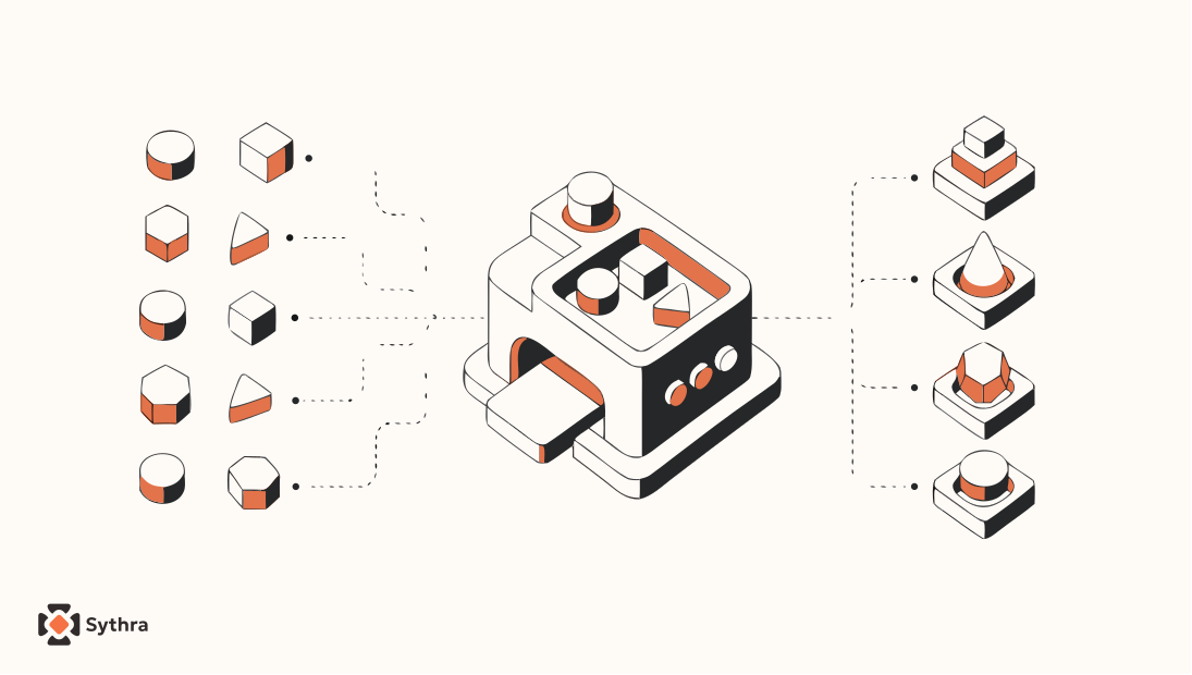
K-Means Clustering is an unsupervised machine learning algorithm designed to partition an unlabeled dataset of observations into distinct, non-overlapping groups (clusters). Because real-world data rarely comes with pre-assigned target labels, K-Means discovers the natural geometric groupings latent within the feature space purely by measuring physical proximity.
1. Key K-Means Concepts & Notation
Before stepping through the optimization formulas, let us establish the formal mathematical notation and terminology used throughout clustering theory:
| Term / Symbol | Mathematical Role | Plain-English Intuition | Impact on Clustering |
|---|---|---|---|
| Number of Clusters () | User-specified hyperparameter: | The target number of groups you instruct the algorithm to discover. | Must be chosen upfront; too small underfits natural clusters, too large fragments them. |
| Centroid () | Mean vector: | The geometric center of mass (the flag) representing cluster . | Acts as the anchor point that defines cluster membership boundaries. |
| Euclidean Distance () | The straight-line ruler distance between a point and a cluster centroid. | Determines which cluster a point belongs to at every iteration. | |
| Assignment Rule | Assigning each person to the nearest meeting flag. | Partitions the dataset into Voronoi cells bounded by perpendicular bisectors. | |
| Inertia / WCSS () | Within-Cluster Sum of Squares: total tightness of all clusters. | The global loss function K-Means seeks to minimize; lower is tighter. | |
| K-Means++ Initialization | Sampling with probability | Planting starting flags as far away from each other as possible. | Guarantees an competitive bound and avoids bad local minima. |
| Silhouette Score () | Measures whether a point is closer to its own cluster than neighboring clusters. | Ranges from (misclustered) to (dense, well-separated cluster). |
2. Mathematical Derivations & Proof of Convergence
K-Means operates as an optimization algorithm that minimizes a single objective function: the Within-Cluster Sum of Squares (WCSS), also known as Inertia:
Where is a -dimensional feature vector, is the set of points assigned to cluster , and is the centroid of cluster . K-Means minimizes this objective using an alternating two-step optimization known as Lloyd's Algorithm (a hard-assignment instance of Expectation-Maximization):
Step 1: The Assignment Phase (Expectation / E-Step)
Holding the centroids fixed, each observation is assigned to its nearest centroid according to squared Euclidean distance:
Because each point independently chooses the centroid that minimizes its individual contribution , this step strictly decreases (or holds constant) the total objective .
Step 2: The Centroid Update Phase (Maximization / M-Step)
Holding the cluster assignments fixed, we recompute each centroid to minimize . To prove why the arithmetic mean is the optimal choice, we compute the partial derivative of with respect to centroid and set it to zero:
This proves analytically that updating to the component-wise arithmetic mean of its assigned observations achieves the unique, global minimum of the squared error for that cluster partition.
3. Worked Numerical Trace (By Hand with 12 Points)
To see the mathematics operating in practice, let us trace an exact execution on a 2D dataset of 12 points grouped into 3 distinct spatial regions:
- Bottom-Left Group (4 points):
- Top-Right Group (4 points):
- Bottom-Right Group (4 points):
Suppose we initialize the three centroids directly on observations , , and :
Iteration 1: Assignment & Centroid Update
Each of the 12 points computes its Euclidean distance to , , and . Because the three groups are widely separated, points assign to , points assign to , and points assign to . We then recompute the centroids:
Iteration 2: Convergence Check & Inertia Calculation
In Iteration 2, every point recalculates distances against the updated centroids. Zero points switch clusters. Because no assignments change, the centroids remain identical, and the algorithm terminates.
Now calculate the exact Within-Cluster Sum of Squares ():
- Cluster 1 WCSS:
- Cluster 2 WCSS:
- Cluster 3 WCSS:
4. From-Scratch Python Implementation (Vectorized NumPy)
Below is a fully vectorized, object-oriented implementation of K-Means built with NumPy. It incorporates tolerance checking, inertia calculation, and safeguards against empty cluster divisions:
import numpy as np

class KMeansScratch:
    """
    K-Means clustering implemented from scratch using NumPy.
    Minimizes Within-Cluster Sum of Squares (WCSS / Inertia).
    """
    def __init__(self, k=3, max_iters=100, tol=1e-4, random_state=42):
        self.k = k
        self.max_iters = max_iters
        self.tol = tol
        self.random_state = random_state
        self.centroids = None
        self.labels = None
        self.inertia_ = None

    def _init_centroids(self, X, rng):
        # Pick k random distinct observations as starting centroids
        indices = rng.choice(len(X), size=self.k, replace=False)
        return X[indices].astype(float).copy()

    def fit(self, X):
        X = np.asarray(X, dtype=float)
        n_samples, n_features = X.shape
        rng = np.random.default_rng(self.random_state)

        self.centroids = self._init_centroids(X, rng)

        for iteration in range(self.max_iters):
            # 1. Assignment Step (E-step): compute distance matrix (n_samples, k)
            # Using Euclidean distance: ||x_i - mu_k||
            distances = np.linalg.norm(X[:, np.newaxis, :] - self.centroids[np.newaxis, :, :], axis=2)
            new_labels = np.argmin(distances, axis=1)

            # 2. Update Step (M-step): recalculate centroids as mean of assigned points
            new_centroids = np.zeros_like(self.centroids)
            for k_idx in range(self.k):
                cluster_members = X[new_labels == k_idx]
                if len(cluster_members) > 0:
                    new_centroids[k_idx] = cluster_members.mean(axis=0)
                else:
                    # Safeguard against empty clusters: re-seed to the point farthest from any centroid
                    furthest_idx = np.argmax(np.min(distances, axis=1))
                    new_centroids[k_idx] = X[furthest_idx]

            # 3. Check for convergence (centroid movement < tolerance)
            centroid_shift = np.linalg.norm(new_centroids - self.centroids)
            self.centroids = new_centroids
            self.labels = new_labels

            if centroid_shift < self.tol:
                break

        # Compute final WCSS (Inertia)
        self.inertia_ = sum(
            np.sum((X[self.labels == k_idx] - self.centroids[k_idx]) ** 2)
            for k_idx in range(self.k)
        )
        return self

    def predict(self, X):
        X = np.asarray(X, dtype=float)
        distances = np.linalg.norm(X[:, np.newaxis, :] - self.centroids[np.newaxis, :, :], axis=2)
        return np.argmin(distances, axis=1)


# Verification test on the 12-point toy dataset
if __name__ == "__main__":
    X = np.array([
        [1.0, 2.0], [1.5, 1.8], [1.0, 0.6], [2.0, 1.0],      # bottom-left group
        [9.0, 11.0], [8.0, 8.0], [9.0, 10.0], [10.0, 9.0],   # top-right group
        [8.0, 2.0], [9.0, 3.0], [10.0, 2.0], [9.0, 1.0],     # bottom-right group
    ])

    model = KMeansScratch(k=3, max_iters=100, random_state=42)
    # Seed centroids directly with initial indices to trace exact hand calculation
    model.centroids = np.array([[1.0, 2.0], [9.0, 11.0], [8.0, 2.0]])
    model.fit(X)

    print("Final Centroids:\n", np.round(model.centroids, 4))
    print("Cluster Labels:", model.labels)
    print(f"Final WCSS (Inertia): {model.inertia_:.4f}")
5. Production Scikit-Learn Pipeline & K-Means++
While naive K-Means picks starting centroids uniformly at random, a poor initial draw can trap the algorithm in an inferior local minimum. To solve this, Arthur and Vassilvitskii (2007) introduced K-Means++, which is the default in Scikit-Learn (init='k-means++').
How K-Means++ Works
- Choose the first centroid uniformly at random from the dataset.
- For every remaining point , compute , the Euclidean distance to the closest centroid already selected.
- Select the next centroid by sampling points with probability proportional to the squared distance:
Repeat steps 2 and 3 until centroids are chosen. By favoring points that are physically far away from existing centroids, K-Means++ spreads the starting seeds across the data manifold, guaranteeing an expected approximation ratio of compared to the global optimal clustering.
import numpy as np
from sklearn.cluster import KMeans
from sklearn.preprocessing import StandardScaler
from sklearn.pipeline import Pipeline
from sklearn.metrics import silhouette_score, silhouette_samples

# 1. Real-world dataset simulation
X = np.array([
    [1.0, 2.0], [1.5, 1.8], [1.0, 0.6], [2.0, 1.0],
    [9.0, 11.0], [8.0, 8.0], [9.0, 10.0], [10.0, 9.0],
    [8.0, 2.0], [9.0, 3.0], [10.0, 2.0], [9.0, 1.0],
])

# 2. Production Pipeline with StandardScaler & K-Means++
# StandardScaler ensures features contribute equally to Euclidean distances
pipeline = Pipeline([
    ("scaler", StandardScaler()),
    ("kmeans", KMeans(n_clusters=3, init="k-means++", n_init=10, random_state=42))
])

pipeline.fit(X)
kmeans_model = pipeline.named_steps["kmeans"]
X_scaled = pipeline.named_steps["scaler"].transform(X)

# 3. Model Evaluation: Inertia & Silhouette Score
labels = kmeans_model.labels_
sil_score = silhouette_score(X_scaled, labels)

print("Cluster Labels:           ", labels)
print(f"Inertia (Scaled WCSS):    {kmeans_model.inertia_:.4f}")
print(f"Silhouette Coefficient:   {sil_score:.4f} (Close to +1 indicates excellent separation)")

# 4. Assessing multiple values of K (Elbow & Silhouette Analysis)
print("\n--- Evaluating K from 2 to 5 ---")
for k in range(2, 6):
    km = KMeans(n_clusters=k, init="k-means++", n_init=10, random_state=42)
    pred_labels = km.fit_predict(X_scaled)
    sil = silhouette_score(X_scaled, pred_labels)
    print(f"K={k} | WCSS (Inertia): {km.inertia_:7.3f} | Silhouette Score: {sil:.3f}")
6. How to Choose K: The Elbow Method vs. Silhouette Analysis
Because K-Means requires specifying upfront, practitioners use two complementary validation techniques to determine the optimal cluster count:
The Elbow Method
The Elbow Method plots WCSS (Inertia) against increasing values of . As increases, inertia naturally decreases (reaching 0 when , where every point is its own centroid). The ideal cluster count corresponds to the 'elbow' inflection point — where adding another cluster yields diminishing marginal returns in variance reduction.
The Silhouette Coefficient
When the elbow curve is smooth and ambiguous, the Silhouette Score provides an objective measure of cluster cohesion and separation for each point :
- : The mean intra-cluster distance from point to all other points in the same cluster (measures compactness).
- : The mean nearest-cluster distance from point to all points in the closest neighboring cluster (measures separation).
- Interpretation: A score near indicates point is well inside its cluster and far from neighbors; indicates on the decision border; indicates point was assigned to the wrong cluster.
| Validation Metric | Primary Advantage | Limitation | Best Use Case |
|---|---|---|---|
| Elbow Method (Inertia) | Fast to compute ( after clustering). | Can be subjective when the curve lacks a sharp bend. | Initial heuristic search across a wide range of values. |
| Silhouette Analysis | Bounded score; evaluates cluster separation directly. | Computationally expensive ( pairwise distances). | Validating exact cluster boundaries on small-to-medium datasets. |
7. When K-Means Fails: 4 Structural Limitations
- Spherical Cluster Assumption: K-Means inherently assumes clusters are isotropic and spherical because it assigns points purely based on Euclidean distance to a single center. If true clusters are elongated ellipses (anisotropic), K-Means will split them incorrectly perpendicular to the long axis (use Gaussian Mixture Models instead).
- Unequal Cluster Sizes & Densities: When one cluster contains 10,000 points and a neighboring cluster contains 50 points, K-Means often pulls the centroid of the small cluster into the dense cloud to minimize total squared error.
- Non-Convex Geometries: Data shaped like concentric rings, interlocking spirals, or crescent moons cannot be separated by K-Means' linear Voronoi boundaries (use DBSCAN or Spectral Clustering).
- Sensitivity to Feature Scales & Outliers: Because squared Euclidean distance penalizes large deviations quadratically, unscaled features dominate distance calculations, and extreme outliers drag centroids far away from true cluster centers.
8. Summary & Key Takeaways
- Unsupervised Clustering: K-Means discovers hidden patterns in unlabeled data by grouping observations around spatial centroids.
- Lloyd's Two-Step Loop: Alternates between assigning points to the closest centroid and updating centroids to the mean of their members.
- Minimizes WCSS: Operates as coordinate descent on Within-Cluster Sum of Squares, guaranteed to converge in a finite number of steps.
- Always Scale Features: Standardization (
StandardScaler) is mandatory so high-magnitude features do not distort distance calculations. - Use K-Means++: Spreads initial seeds using distance weighting, avoiding sub-optimal local minima traps.
Common questions
Why is K-Means called an unsupervised machine learning algorithm?
K-Means is unsupervised because it does not require target labels, ground truth classes, or teacher feedback during training. It discovers natural groupings purely through the intrinsic geometric distances between data points in feature space.
How does K-Means++ improve on standard random initialization?
Standard K-Means picks starting centroids uniformly at random, which often places multiple centroids in the same cluster. K-Means++ chooses the first centroid randomly, then samples subsequent centroids with probability proportional to the squared distance from existing centroids (D(x)^2). This forces initial seeds to spread across the entire dataset, accelerating convergence and guaranteeing an O(log K) bound against the global optimum.
Why is feature scaling mandatory before running K-Means?
K-Means relies strictly on Euclidean distance (sqrt(sum((x_i - mu_k)^2))). If one feature ranges from 0 to 1 (like age ratio) and another ranges from 0 to 100,000 (like annual income), the larger feature will dominate the distance calculations by orders of magnitude, effectively rendering the smaller feature invisible.
How do you find the best value for K in K-Means?
The two primary methods are the Elbow Method and Silhouette Analysis. The Elbow Method plots WCSS (inertia) across multiple K values to identify where the rate of variance reduction sharply slows down. Silhouette Analysis measures how well-separated clusters are on a scale from -1 to +1, helping disambiguate smooth elbow curves.
What is the key difference between K-Means and KNN (K-Nearest Neighbors)?
Despite similar names, they solve opposite tasks: K-Means is an unsupervised clustering algorithm that groups unlabeled data into K clusters. KNN is a supervised classification and regression algorithm that predicts labels for new test queries based on the majority vote of their K nearest labeled training neighbors.
Explore
Related topics
Keep going — these sit next to this concept in a real learning path.
K-Nearest Neighbors (KNN) in Python From Scratch
Master Euclidean distance metrics and nearest-neighbor lookups in classification.
Supervised vs Unsupervised Learning: The Math and Code
Understand the foundational differences between labeled prediction and latent pattern discovery.
Handling Imbalanced Datasets: SMOTE and Class Weighting
Learn how nearest-neighbor topology is used to synthesize balanced training distributions.
Exploratory Data Analysis in Python: Complete Walkthrough
Explore data distributions, feature scaling, and cluster visualization in Python.